Distinction in Computational Fluid Dynamics from Cranfield University. Thesis title: "Vorticity Formulations for Predicting the Flow of an Incompressible Fluid".
The model is trained on the training data.
Its ability to predict the correct outcome for
new unseen examples is called it's ability
to generalise.
Overfitting is when too many features are added, and interpolating
causes wild prediction. This is also called high variance.
You can have a situation where the cost is zero but the outcomes
predicted are incorrect. We can look at the problem of over-fitting
in the context of linear regression or logistic regression (classification problems).
Overfitting
Solutions to overfitting include:
Collect more data
Reduce features (Feature Selection)
Reduce size of parameters (Regularisation)
Lots of features with little training data can cause overfitting.
It is not always clear whether the model is under or over-fitting.
Features could include, say, size of house, number of bedrooms, in
a house price prediction model. Some features might be more impactful
than others. This is why we do feature selection. If the model is overfitting, first you would try to source
more training data, but this is not always possible. You could reduce
features, but then you risk losing information. In that case you
would want to remove the least impactful features, but it might not
be clear which those are. This is why the other option regularisation
is often used.
This means to reduce the size of certain parameters, and is quite common.
Regularisation of the b parameter is usually negligible.
Ground Truth Data Ltd are building synthetic data pipelines
to supply healthcare ML companies with training and evaluation data.
The company was co-founded by myself, Dr Tamas Jozsa, Tianyu Ma,
and Muhammad Gillani.
Our first product is our Synstro technology.
This uses mechanistic methods, combining our expertise
in computational methods and cerebral mechanics,
to generate synthetic CT and MR imaging.
This data is used to train and evaluate models and
to increase model performance.
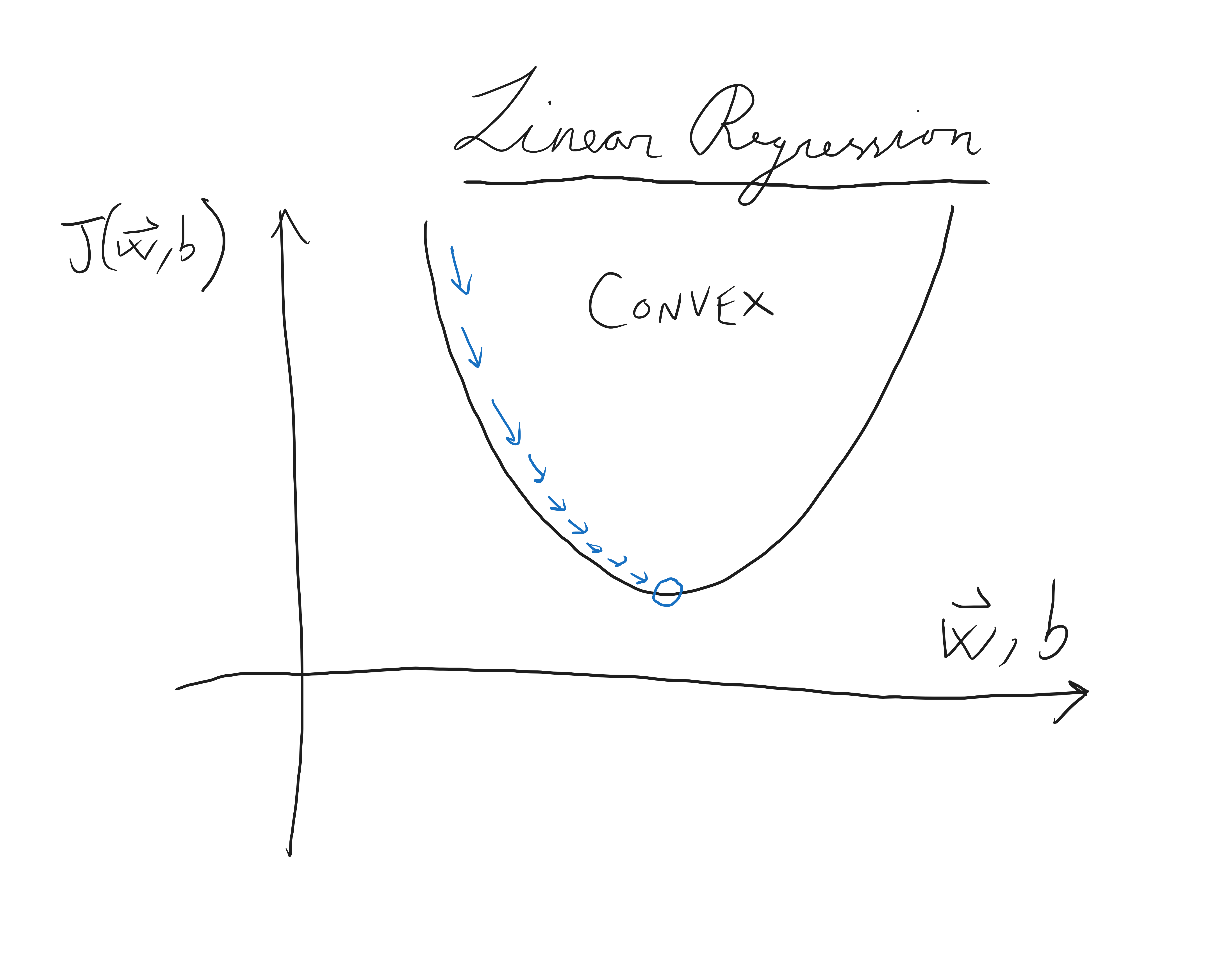
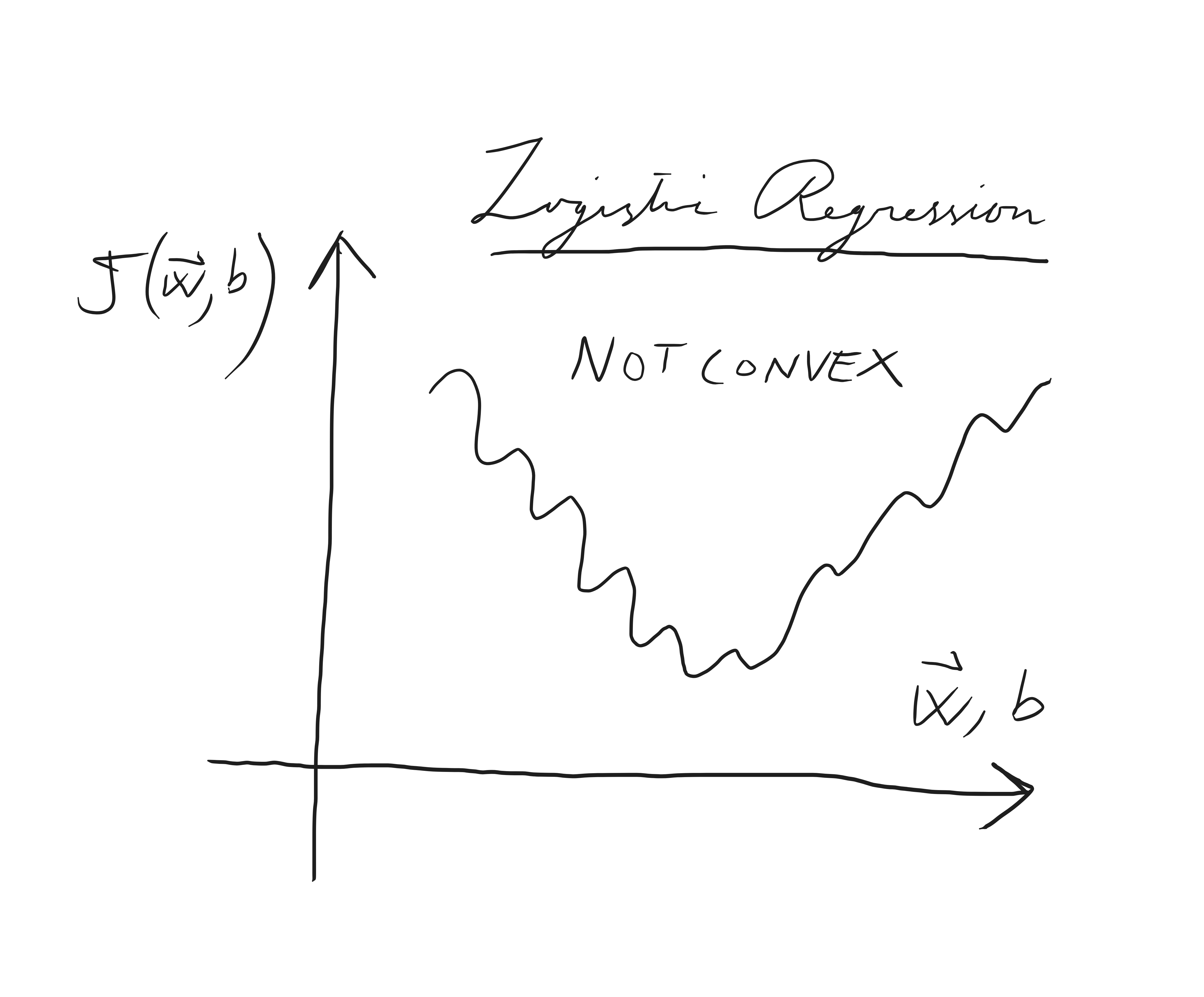
For Logistic Regression, this cost function is not convex, which means
gradient descent is not optimal. For Logistic Regression we require
a different cost function.
Linear Regression with a Square-Error Cost Function
Logistic Regression with a Square-Error Cost Function
This is derived from statistics using maximum likelihood estimation.
What does this loss function mean? It basically means you punish the cost function harder
the further your predicted value is from the true value. And it occurs to me
that you could optimise this loss function further.
The loss function for logistic regression can be written as a single equation,
Classification problems have binary or discrete outcomes.
For example, a tumour can be identified as either benign or malignant.
An email can be identified as either spam or not spam.
These are called binary classification problems.
However, there may be more than one class or category into
which the data may fall. And although the output may be discrete, the
input can be continuous.
A threshold then has to be decided in order to determine which data are in
which category. Linear regression does not usually work well for classification
problems. That is, a linear model is insufficient to model categorical data.
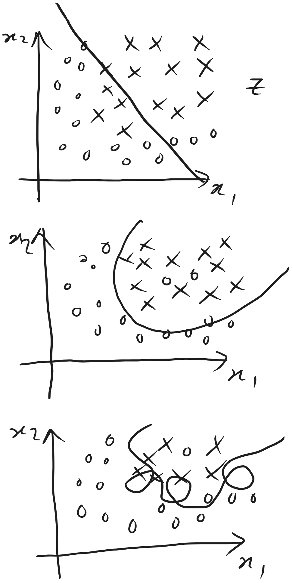
Because a linear fit is not usually good enough in this case, a sigmoid
function, also known as 'logistic regression' is often used to define the threshold. The threshold may also be adjusted,
for example you are likely to lower the threshold if you are identifying tumours as
you would not want to miss one. We then get a decision boundary,
and decision boundaries can vary in complexity, up to and including complex polynomials.
Let's say we have two continuous variables, size and colour, of a tumour. And let's say we have some amount of data
that has been collected, size of tumour, colour of tumour, and whether the outcome was benign or malignant. We can train
a model on this data, but it will be a classification problem, because the outcome is either benign or malignant.
So we need to decide a threshold for what exact combination of colour and size can distinguish between benign or
malignant. To do this, we train a logistic regression model on the training set to determine a decision boundary.
The decision boundary can be a complicated function.
and the \(\textbf{x}\) vector is the feature vector (for colour, size etc.),
\(\textbf{w}\) is the parameter vector, \(b\) is another parameter, and \(i\) is the
\(i\)th training sample in the training set of size \(m\).
The output of this function
can be interpreted as the probability that the outcome is 'yes' or 1. The sigmoid
function is acting like a transformation, keeping the output of the linear regression model
between 0 and 1,
\[f_{w.b} (\textbf{x}^{(i)}) = g(\textbf{w} \cdot \textbf{x}^{(i)} + b) = P(y=1|\textbf{x};\textbf{w},b)\]
Here we can alter the threshold determining whether our prediction \(\hat{y}\) is 'yes' vs 'no' as we see fit depending on the application.
However, in this case, the function is non-linear so the squared-error cost function
which was used previously to find the best parameters does not lead to effective gradient descent. Therefore we need a
new cost function.
This worked well for linear regression but it will not work well for
logistic regression. It leads to a cost function which is not smooth and not easy for gradient descent,
because the function \(f\) is non-linear,
Andrew Ng's Course: Feature Engineering and Polynomial Regression
9th May 2026
This is continuuing Andrew Ng's course in Machine Learning Specialization.
The linear fit or the linear model is not necessarily always the best fit
to the training data.
If the training data has curvature, we probably need some higher order terms in
the fit.
Oftentimes a polynomial fit is better.
We can, therefore, add more features to the model, including quadratic
and cubic terms.
Gradient descent will then determine which feature is most important by adjusting
the parameters accordingly.
Another important point is feature engineering or feature scaling. This means adjusting the ranges of the features:
if there is a large difference in the range of each feature, such as \(x\) and \(x^2\), we apply z-score normalisation to the features and this speeds up gradient descent.
We can continue to add a number of features, and gradient
descent will identify which are most important by the size of the corresponding parameter.
We can also identify the best features by using linear regression; seeing if the new feature is linear w.r.t the target.
This is a valuable video by one of the key machine learning figures, Andrej Karpathy.
Although it is now out of date by one year. At first I thought, how hard can it be to type a prompt into and LLM an get a result?
But there are some useful tips in how to use these powerful tools effectively in this
video. It also helps to have some insight into how the models work as this allows you to
make the best use their capabilities. Link to the video:
https://www.youtube.com/watch?v=EWvNQjAaOHw
The context window
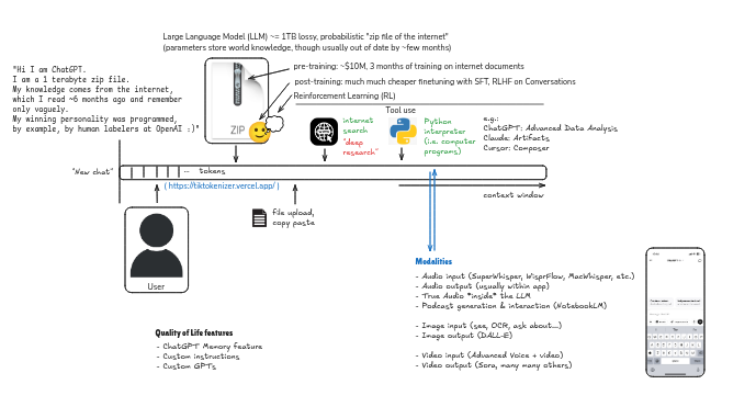
Before recalling information from the video, it is important to note that Large Language Models (LLMs) are
just one manifestation of artifical intelligence. They are text-based. This is the most popular format of AI due to the
fact that ChatGPT went viral and that it is easy for users to use and understand.
The most valuable detail to consider with LLMs is the idea of the 'context window'. Every new chat refreshes the context window.
This is the important to note as any new topic ought to be started in a new chat. The model has the entire context window available to it
when it predicts the next token in a new response.
Another thing to note is that the chat mode, which looks like Whatsapp or iMessage, is superficial. Both the user query and the response go into a
single train of tokens, and they build up a one-dimensional context window.
The text in the user query and the response is chopped up into tokens which are essentially a set of unique identifiers identifying that symbol.
The text is chopped into tokens and coded with numbers so that the context window is just a one-dimensional stream of tokens or numbers.
The model in Andrew Ng's lessons was the 'linear regression model', a fit to the data which uses gradient descent to minimise a cost function.
The model in LLMs is a much more advanced version of this, but it is still just trying to predict the next token.
To get a valuable, functional, advanced model, lots of training data on language and text is needed. These advanced LLM models are trained on a training set
of the entire internet. The internet is chopped up into tokens, and this is used to train the model to predict the next token in a response. So ChatGPT is just a 1Tb zip file of the
whole internet as it was ~6 months ago. The training phase is called 'pre-training', and it is long and expensive -
we are talking months and billions of dollars. Therefore, the information which the models
have access to is outdated and the model's recall of the internet is probabilistic and 'lossy'.
Tool-use has changed this, because now most models have
the capacity to search the internet.
It is also important to remember that the model may hallucinate at any time.
Post-training comes after, and this is where the knowledge of the internet the model has is granted a character, a human-like character,
and knowledge of conversation. This gives the model style and makes them more usable.
Functionality of the LLMs has also grown over time. 'Thinking' mode uses reinforcement learning. There are also 'deep research' functions.
One use case Karpathy highlights is as an aid to reading. You may submit pdfs or text to the model in the context window and it will use it
as context. This is a valuable tool. The model can summarise papers, books, chapters. This saves lots of time reading papers for academics,
or reading books in general. I think this is one of the most valuable use cases of LLMs which I have learnt from Karpathy.
Tool use changes the game. Models can run Python code to do calculations. They can search webpages.
One year ago when Karpathy made this video, computer-use was spoken about but not yet available.
Computer-use changes the game again. And now we have autonomous agents with computer-use.
This is causing and will cause crazy acceleration.
Most large labs now seem to be focused on code-gen, because code-gen is upstream of everything.
This explains XAI's aquisition of Cursor, as Grok was lagging behind on code-gen.
Gradient descent is key and a general minimisation algorithm.
Gradient descent helps us to identify optimal values of \(w\) and \(b\) in order to minimise \(J(w,b)\)
as opposed to just trial and error.
On a 3D landscape of hills and valleys it will move us towards the local minima.
Gradient descent algorithm: repeat the following until convergence,
\[w = w - \alpha \frac{\partial}{\partial w} J(w,b)\]
\[b = b - \alpha \frac{\partial}{\partial b} J(w,b)\]
Andrew Ng's Course: Machine Learning Specialization
28th April 2026
I have enrolled in Andrew Ng's 'Machine Learning Specialization' course.
Here's what I did so far.
Supervised learning involves teaching the machine with reference to historical data.
We are essentially optimising some function.
The more training data, the better our function will fit new data. To teach the machine, we create learning algorithms.
Learning algorithms alter the parameters of the chosen model to better match the data.
Specifically, they work to minimise a cost function. That is, we are fitting a model (a function) to
the data by altering parameters to find the local minima of the cost function. With two parameters in
the model, the cost function is a 3D sheet.
Supervised learning is teaching the algorithm to match x to y, input to output, using lots of examples of
'right answers'. It is helpful to think of what we are doing at the most basic level as
producing an output for some given input. Google Translate takes English as input and outputs Spanish.
A self-driving care takes image and lidar data as input, and outputs the position of a passing car. Gmail takes
the email as input, and outputs yes/no to whether it is spam.
In a sense you can summarise all computing as matching an input to
an output. The question is, can you teach the machine to do that autonomously.
Supervised learning, using examples of 'right answers', can use regression or classification. Regression
aims to output a number from infinitely many numbers. Classification aims to output a class/category from
a small number of possible outputs.
Unsupervised learning finds structures or patterns in the new data by itself. This can be used for clustering, such as Apple News
clustering articles together. It can also be used for grouping, such as for grouping your customers to understand who is using
your product.
So we feed a training set to a learning algorithm, and it produces the function/model f which will take input x and produce estimated output y_hat.
This function might be linear. To start, let's assume it is linear. Then is has some constant b, and some gradient w. We can denote the training set
as (x,y) and training example as (x_i, y_i). Let's say the model is a linear function:
\[ f_{w,b} (x) = wx + b \]
here \(w\) and \(b\) are the parameters/weights/coefficients.
The cost function, \( J(w,b) \), is the difference between predicted \(\hat{y}^{(i)}\) and \(y^{(i)}\), quantified:
where \(m\) is the number of training examples in the training set. This is the squared-error cost function.
Our job is to find \(w\), \(b\), such that \(\hat{y}^{(i)}\) is close to \(y^{(i)}\) for all \((x^{(i)}, y^{(i)})\). Recall,
\[\hat{y}^{(i)} = f_{w,b}(x^{(i)})\]
that is to say predicted values come from our model or function. Then,
This is a simple project, but one that I found interesting as it occurred to me that LLM's probably have a similar process.
The code takes as input any text, and returns the corresponding reading level (for education purposes).
This involves counting the letters, words, and sentences, then applying an algorithm to infer reading level.
I guess the machine learning would optimise that algorithm by supervised training.
I imagine that LLM's apply statistics to discover relationships
between the words and letters and sentences, incorporating machine learning which is trained for spotting the
patterns between them.
There must be two steps. 1. Intepreting the user's prompt, which is something similar to assessing the reading level of the input text
2. Constructing an appropriate response.
Where the Coleman-Liau index was applied, a machine learning algorithm will have produced a similar equation.
Or, the machine learning would be used to get the Coleman-Liau equation, using known data.
                    # Returns the reading level of any text

                    from cs50 import get_string

                    def main():
                        # Get text from the user
                        text = get_string("Text: ")

                        # Count letters in the text
                        letter_count = count_letters(text)

                        # Count words in the text
                        word_count = count_words(text)

                        # Count sentences in the text
                        sentence_count = count_sentences(text)

                        # Calculate reading level
                        avg_letters = (letter_count / word_count) * 100

                        avg_sentences = (sentence_count / word_count) * 100

                        reading_level = coleman_liau(avg_letters, avg_sentences)

                        # Print reading level between 1 and 16
                        if 1 <= reading_level < 16:
                            print(f"Grade {round(reading_level)}")
                        elif reading_level < 1:
                            print("Below Grade 1")
                        elif reading_level > 16:
                            print("Grade 16+")


                    def count_letters(text):
                        letter_count = 0
                        for character in text.lower():
                            if character.isalpha():
                                letter_count += 1
                        return letter_count


                    def count_words(text):
                        word_count = 1
                        for character in text:
                            if character == " ":
                                word_count += 1
                        return word_count


                    def count_sentences(text):
                        sentence_count = 0
                        for character in text:
                            if character in ".?!":
                                sentence_count += 1
                        return sentence_count

                    def coleman_liau(avg1, avg2):
                        level = 0.0588 * avg1 - 0.296 * avg2 - 15.8
                        return level


                    if __name__ == "__main__":
                        main()
Currently working on incompressible solvers and advancing the vector potential-vorticity method.
Writing the Pressure-Poisson approach for a simple case.
Eventually, will focus on the artificial compressibility approach because you can use Godunov methods
and solve discontinuities. In this case the governing equations are hyperbolic.
I worked on incompressible flow modelling for my thesis at Cranfield. That means you
can neglect density variation of the fluid medium, which usually means
low speed.
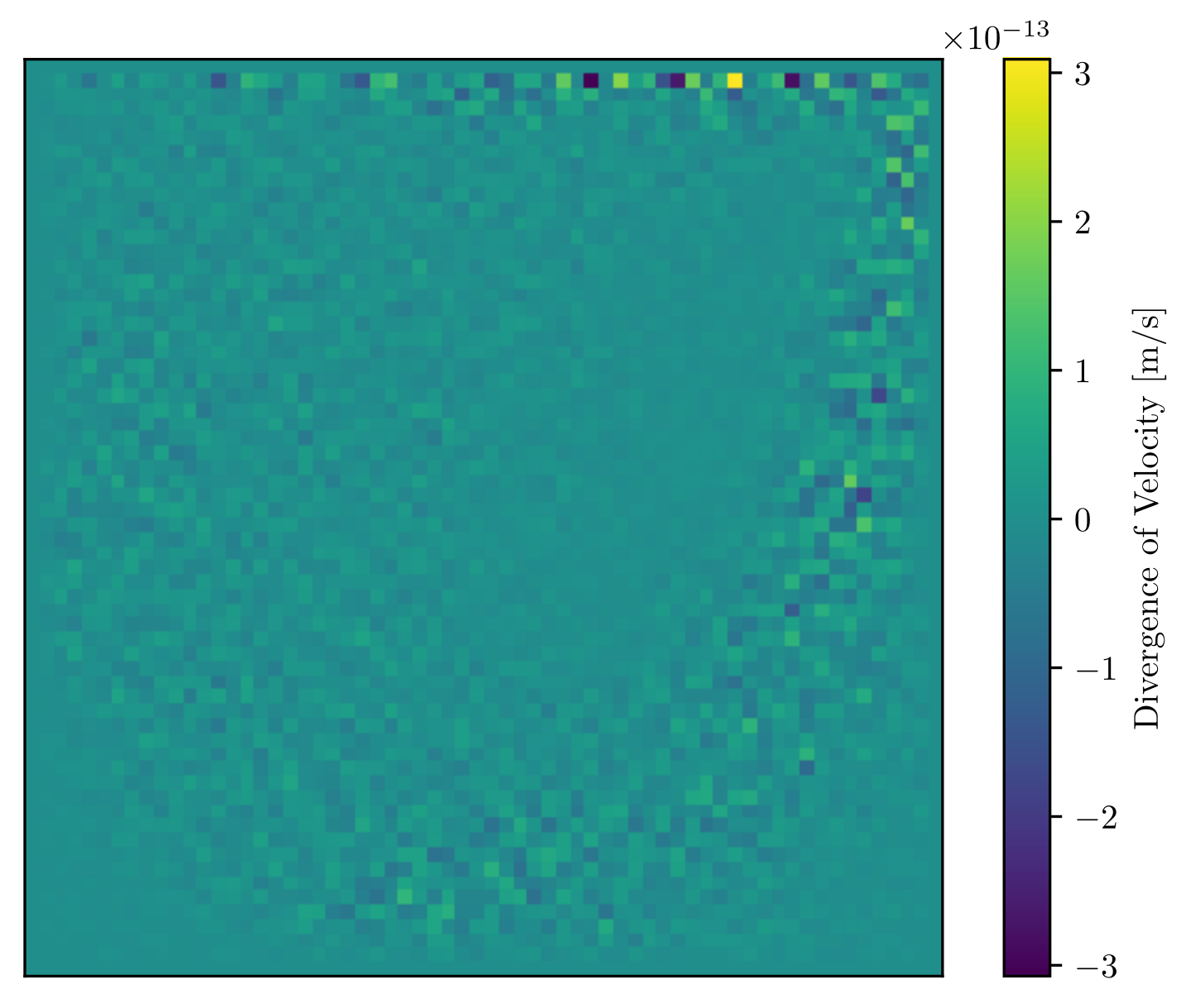
It means the divergence of velocity is zero. This is kind of an ideal, pure
mathematical system which can sometimes be used to map reality accurately.
I wrote the streamfunction-vorticity formulation first,
which is only applicable to two dimensions.
This is because the streamfunction only exists in two dimensions.
I validated the results produced by my code using the lid-driven
square cavity benchmark (2D), comparing centreline velocities.
The figure above shows divergence of velocity for the vector potential-vorticity
formulation. It is a slice of the centreplane of a cube,
where the cube is full of continuous fluid, and the lid is
moving from left to right. This is a standard benchmark against
which to test the results of your code.
The results are well-known. In both
the streamfunction-vorticity formulation (2D) and the
vector-potential vorticity formulation (3D), the divergence of
velocity is satisfied explicitly. Hence why divergence
above is small. This is the advantage of
vorticity formulations over, say, the primitive variable
approach. The main focus of my thesis was the
vector-potential vorticity formulation, which is harder to
implement. This method requires more work to be
workable.
In layman's terms:
Imagine a solid cube full of any fluid - air, water,
Coca-Cola. Now imagine moving the upper surface in some direction.
How would the fluid in the container move? What pattern would it
make? Solving a complex equation approximately, with the aid
of a computer, allows you predict what the patterns would be.
You can say, at any point in the cube (for the most part),
and even at any particular instance in time, precisely
what the temperature, pressure, speed, and direction of
motion of the fluid will be. The resulting
pattern that your code produces, can be compared against
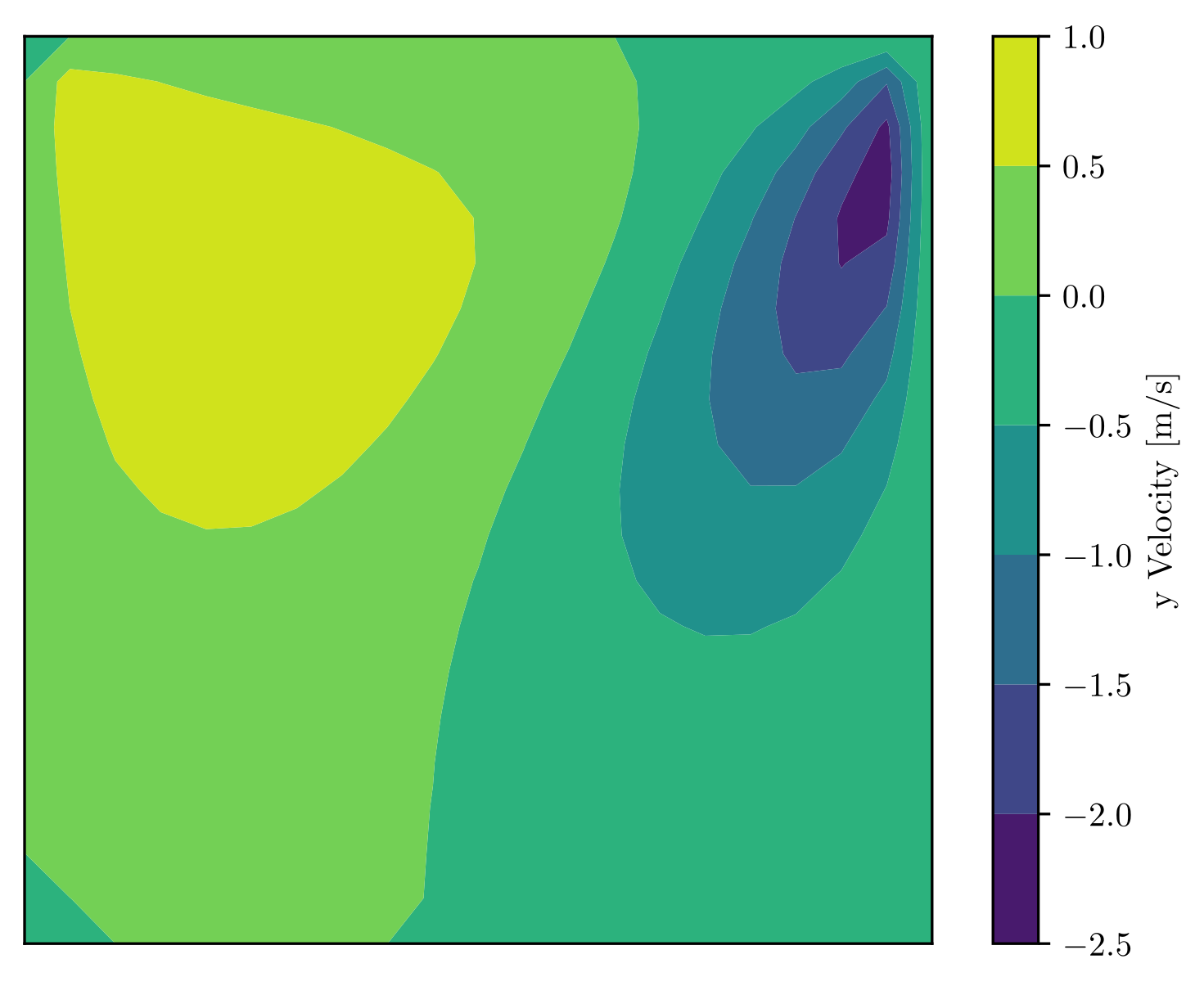
experiments, so you can check it's true. Here's one
such pattern:
What does this show?
The speed of motion of the fluid in the up and down direction,
on a cross-section of the cube along the centreplane. Lid motion
is from left to right.